The material we covered in the last two posts (skin friction and pressure drag) allows us to consider a fun little problem:
How quickly do the small bubbles of gas rise in a pint of beer?
To answer this question we will use the concept of aerodynamic drag introduced in the last two posts – namely,
- skin friction drag – frictional forces acting tangential to the flow that arise because of the inherent stickiness (viscosity) of the fluid.
- pressure drag – the difference between the fluid pressure upstream and downstream of the body, which typically occurs because of boundary layer separation and the induced turbulent wake behind the body.
The most important thing to remember is that both skin friction drag and profile drag are influenced by the shape of the boundary layer.
What is this boundary layer?
As a fluid flows over a body it sticks to the body’s external surface due to the inherent viscosity of the fluid, and therefore a thin region exists close to the surface where the velocity of the fluid increases from zero to the mainstream velocity. This thin region of the flow is known as the boundary layer and the velocity profile in this region is U-shaped as shown in the figure below.
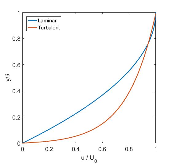
Velocity profile of laminar versus turbulent boundary layer
As shown in the figure above, the flow in the boundary layer can either be laminar, meaning it flows in stratified layers with no to very little mixing between the layers, or turbulent, meaning there is significant mixing of the flow perpendicular to the surface. Due to the higher degree of momentum transfer between fluid layers in a turbulent boundary layer, the velocity of the flow increases more quickly away from the surface than in a laminar boundary layer. The magnitude of skin friction drag at the surface of the body (y = 0 in the figure above) is given by

where 
Skin friction drag is the dominant form of drag for objects whose surface area is aligned with the flow direction. Such shapes are called streamlined and include aircraft wings at cruise, fish and low-drag sports cars. For these streamlined bodies it is beneficial to maintain laminar flow over as much of the body as possible in order to minimise aerodynamic drag.
Conversely, pressure drag is the difference between the fluid pressure in front of (upstream) and behind (downstream) the moving body. Right at the tip of any moving body, the fluid comes to a standstill relative to the body (i.e. it sticks to the leading point) and as a result obtains its stagnation pressure.
The stagnation pressure is the pressure of a fluid at rest and, for thermodynamic reasons, this is the highest possible pressure the fluid can obtain under a set of pre-defined conditions. This is why from Bernoulli’s law we know that fluid pressure decreases/increases as the fluid accelerates/decelerates, respectively.
At the trailing edge of the body (i.e. immediately behind it) the pressure of the fluid is naturally lower than this stagnation pressure because the fluid is either flowing smoothly at some finite velocity, hence lower pressure, or is greatly disturbed by large-scale eddies. These large-scale eddies occur due to a phenomenon called boundary layer separation.
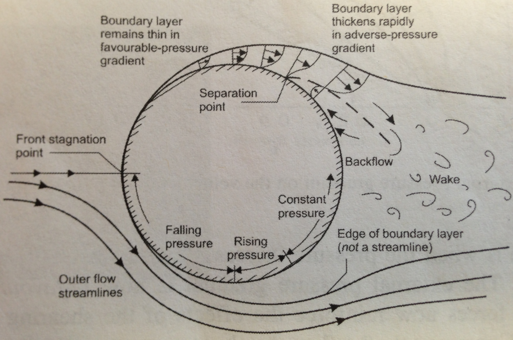
Boundary layer separation over a cylinder
Why does the boundary layer separate?
Any body of finite thickness will force the fluid to flow in curved streamlines around it. Towards the leading edge this causes the flow to speed up in order to balance the centripetal forces created by the curved streamlines. This creates a region of falling fluid pressure, also called a favourable pressure gradient. Further along the body, the streamlines straighten out and the opposite phenomenon occurs – the fluid flows into a region of rising pressure, also known as an adverse pressure gradient. This adverse pressure gradient decelerates the flow and causes the slowest parts of the boundary layer, i.e. those parts closest to the surface, to reverse direction. At this point, the boundary layer “separates” from the body and the combination of flow in two directions induces a wake of turbulent vortices; in essence a region of low-pressure fluid.
The reason why this is detrimental for drag is because we now have a lower pressure region behind the body than in front of it, and this pressure difference results in a force that pushes against the direction of travel. The magnitude of this drag force greatly depends on the location of the boundary layer separation point. The further upstream this point, the higher the pressure drag.
To minimise pressure drag it is beneficial to have a turbulent boundary layer. This is because the higher velocity gradient at the external surface of the body in a turbulent boundary layer means that the fluid has more momentum to “fight” the adverse pressure gradient. This extra momentum pushes the point of separation further downstream. Pressure drag is typically the dominant type of drag for bluff bodies, such as golf balls, whose surface area is predominantly perpendicular to the flow direction.
So to summarise: laminar flow minimises skin-friction drag, but turbulent flow minimises pressure drag.
Given this trade-off between skin friction drag and pressure drag, we are of course interested in the total amount of drag, known as the profile drag. The propensity of a specific shape in inducing profile drag is captured in the dimensionless drag coefficient

where 


The denominator of the drag coefficient represents the dynamic pressure of the fluid (

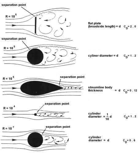
Skin friction drag versus pressure drag for differently shaped bodies
Looking at the diagram above we can start to develop an appreciation for the relative magnitude of pressure drag and skin friction drag for different bodies. The “worst” shape for boundary layer separation is a plate perpendicular to the flow as shown in the first diagram. In this case, drag is clearly dominated by pressure drag with negligible skin friction drag. The situation is similar for the cylinder shown in the second diagram, but in this case the overall profile drag is smaller due to the greater degree of streamlining.
The degree of boundary layer separation, and therefore the wake of eddies behind the cylinder, depends to a large extent on the surface roughness of the body and the Reynolds number of the flow. The Reynolds number is given by

where 

This influence of Reynolds number can be observed by comparing the second diagram to the bottom diagram. The flow over the cylinder in the bottom diagram has increased by a factor of 100 (


Notice also that the streamlined aircraft wing shown in the third diagram has a much lower drag coefficient. This is because the aircraft wing is essentially a “drawn-out” cylinder of the same “thickness”
Terminal velocity of rising beer bubbles
The terminal velocity is the speed at which the forces accelerating a body equal those decelerating it. For example, the aerodynamic drag acting on a sky diver is proportional to the square of his/her falling velocity. This means that at some point the sky diver reaches a velocity at which the drag force equals the force of gravity, and the sky diver cannot accelerate any further. Hence, the terminal velocity represents the velocity at which the forces accelerating a body are equal to those decelerating it.
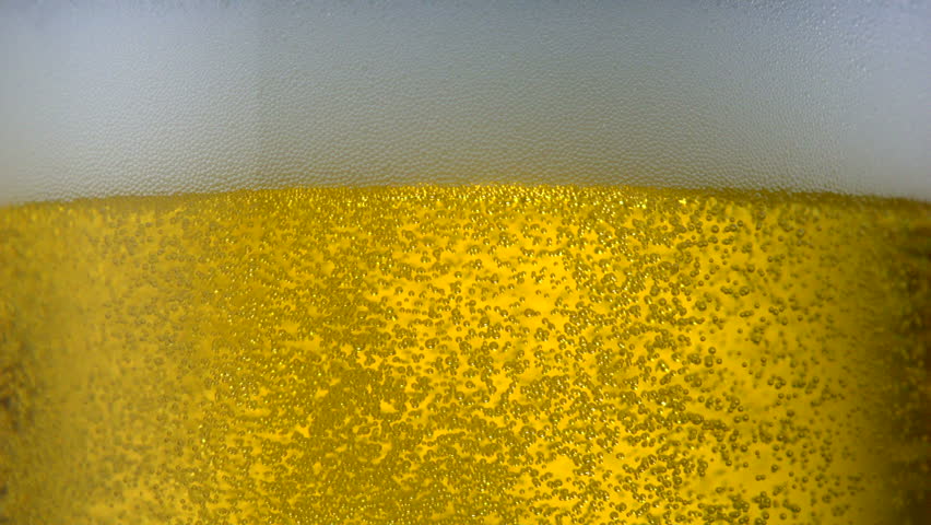
Beer bubbles rising to the surface

Turbulent wake behind a moving sphere. We will model the gas bubbles rising to the top of beer as a sphere moving through a liquid
The net accelerating force of a bubble of air/gas in a liquid is the buoyancy force, i.e. the difference in density between the liquid and the gas. This buoyancy force 
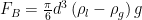
where 


At terminal velocity the buoyancy force is balanced by the total drag acting on the gas bubble. Using the equation for the drag coefficient above we know that the total drag 
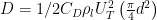
where 


and re-arranging for terminal velocity gives us
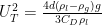
At this point we can calculate the terminal velocity of a spherical gas bubble driven by buoyancy forces for a certain drag coefficient. The problem now is that the drag coefficient of a sphere is not constant; it changes with the flow velocity. Fortunately, the drag coefficient of a sphere plateaus at around 0.5 for Reynolds numbers 

Drag coefficient as a function of Reynolds number. The curve flattens out between 10^3 and 10^5.
 and density of the fluid equal to
  (5% volume beer).
Therefore, the terminal velocity of gas bubbles rising in a beer are somewhere in the range of

and taking the square root

Given that the viscosity of the fluid is around 
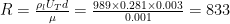
which is right at the bottom of R =
So there you have it: Beer bubbles rise at around a foot per second.
Perhaps the next time you gaze pensively into a glass of beer after a hard day’s work, this little fun-fact will give you something else to think (or smile) about.
Acknowledgements
This post is based on a fun little problem that Prof. Gary Lock set his undergraduate students at the University of Bath. Prof. Lock was probably the most entertaining and effective lecturer I had during my undergraduate studies and has influenced my own lecturing style. If I can only pass on a fraction of the passion for engineering and teaching that Prof. Lock instilled in me, I consider my job well done.

I actually proposed this as my ME senior project at MSOE in 1988, after a night out drinking with classmates. Fortunately, or unfortunately, I was talked into examining the drag of spheres dropping in a column of liquid (not beer). It was a success, but not as interesting as studying bubbles in fluid or beer. I looked this study up after discussing my project with a coworker thirty two years later. I’ve only browsed the article, but will return for a deeper read. I like what I’ve read so far.