On Boundary Layers: Laminar, Turbulent and Skin Friction

On September 18, 2016 · In Aerodynamics, General Aerospace

In the early 20th century, a group of German scientists led by Ludwig Prandtl at the University of Göttingen began studying the fundamental nature of fluid flow and subsequently laid the foundations for modern aerodynamics. In 1904, just a year after the first flight by the Wright brothers, Prandtl published the first paper on a new concept, now known as the boundary layer. In the following years, Prandtl worked on supersonic flow and spent most of his time developing the foundations for wing theory, ultimately leading to the famous red triplane flown by Baron von Richthofen, the Red Baron, during WWI.

Prandtl’s key insight in the development of the boundary layer was that as a first-order approximation it is valid to separate any flow over a surface into two regions: a thin boundary layer near the surface where the effects of viscosity cannot be ignored, and a region outside the boundary layer where viscosity is negligible. The nature of the boundary layer that forms close to the surface of a body significantly influences how the fluid and body interact. Hence, an understanding of boundary layers is essential in predicting how much drag an aircraft experiences, and is therefore a mandatory requirement in any first course on aerodynamics.

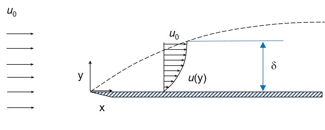
Boundary layers develop due to the inherent stickiness or viscosity of the fluid. As a fluid flows over a surface, the fluid sticks to the solid boundary which is the so-called “no-slip condition”. As sudden jumps in flow velocity are not possible for flow continuity requirements, there must exist a small region within the fluid, close to the body over which the fluid is flowing, where the flow velocity increases from zero to the mainstream velocity. This region is the so-called boundary layer.

The U-shaped profile of the boundary layer can be visualised by suspending a straight line of dye in water and allowing fluid flow to distort the line of dye (see below). The distance of a distorted dye particle to its original position is proportional to the flow velocity. The fluid is stationary at the wall, increases in velocity moving away from the wall, and then converges to the constant mainstream value $u_0$ at a distance $\delta$ equal to the thickness of the boundary layer.

To further investigate the nature of the flow within the boundary layer, let’s split the boundary layer into small regions parallel to the surface and assume a constant fluid velocity within each of these regions (essentially the arrows in the figure above). We have established that the boundary layer is driven by viscosity. Therefore, adjacent regions within the boundary layer that move at slightly different velocities must exert a frictional force on each other. This is analogous to you running your hand over a table-top surface and feeling a frictional force on the palm of your hand. The shear stresses $\tau$ inside the fluid are a function of the viscosity or stickiness of the fluid $\mu$ , and also the velocity gradient $du/dy$ :

$\tau = \mu \frac{\mathrm{d}u}{\mathrm{d}y}$

where $y$ is the coordinate measuring the distance from the solid boundary, also called the “wall”.

Prandtl first noted that shearing forces are negligible in mainstream flow due to the low viscosity of most fluids and the near uniformity of flow velocities in the mainstream. In the boundary layer, however, appreciable shear stresses driven by steep velocity gradients will arise.

So the pertinent question is: Do these two regions influence each other or can they be analysed separately?

Prandtl argued that for flow around streamlined bodies, the thickness of the boundary layer is an order of magnitude smaller than the thickness of the mainstream, and therefore the pressure and velocity fields around a streamlined body may analysed disregarding the presence of the boundary layer.

Eliminating the effect of viscosity in the free flow is an enormously helpful simplification in analysing the flow. Prandtl’s assumption allows us to model the mainstream flow using Bernoulli’s equation or the equations of compressible flow that we have discussed before, and this was a major impetus in the rapid development of aerodynamics in the 20th century. Today, the engineer has a suite of advanced computational tools at hand to model the viscid nature of the entire flow. However, the idea of partitioning the flow into an inviscid mainstream and viscid boundary layer is still essential for fundamental insights into basic aerodynamics.

Laminar and turbulent boundary layers

One simple example that nicely demonstrates the physics of boundary layers is the problem of flow over a flat plate.

Development of boundary layer over a flat plate including the transition from a laminar to turbulent boundary layer.

The fluid is streaming in from the left with a free stream velocity $U_0$ and due to the no-slip condition slows down close to the surface of the plate. Hence, a boundary layer starts to form at the leading edge. As the fluid proceeds further downstream, large shearing stresses and velocity gradients develop within the boundary layer. Proceeding further downstream, more and more fluid is slowed down and therefore the thickness, $\delta$ , of the boundary layer grows. As there is no sharp line splitting the boundary layer from the free-stream, the assumption is typically made that the boundary layer extends to the point where the fluid velocity reaches 99% of the free stream. At all times, and at at any distance $x$ from the leading edge, the thickness of the boundary layer $\delta$ is small compared to $x$ .

Close to the leading edge the flow is entirely laminar, meaning the fluid can be imagined to travel in strata, or lamina, that do not mix. In essence, layers of fluid slide over each other without any interchange of fluid particles between adjacent layers. The flow speed within each imaginary lamina is constant and increases with the distance from the surface. The shear stress within the fluid is therefore entirely a function of the viscosity and the velocity gradients.

Further downstream, the laminar flow becomes unstable and fluid particles start to move perpendicular to the surface as well as parallel to it. Therefore, the previously stratified flow starts to mix up and fluid particles are exchanged between adjacent layers. Due to this seemingly random motion this type of flow is known as turbulent. In a turbulent boundary layer, the thickness $\delta$ increases at a faster rate because of the greater extent of mixing within the main flow. The transverse mixing of the fluid and exchange of momentum between individual layers induces extra shearing forces known as the Reynolds stresses. However, the random irregularities and mixing in turbulent flow cannot occur in the close vicinity of the surface, and therefore a viscous sublayer forms beneath the turbulent boundary layer in which the flow is laminar.

An excellent example contrasting the differences in turbulent and laminar flow is the smoke rising from a cigarette.

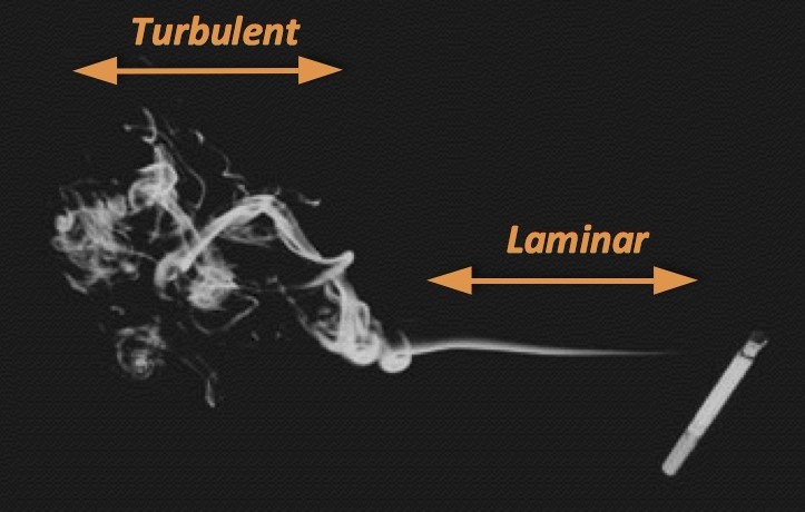
Laminar and turbulent flow in smoke

As smoke rises it transforms from a region of smooth laminar flow to a region of unsteady turbulent flow. The nature of the flow, laminar or turbulent, is captured very efficiently in a single parameter known as the Reynolds number

$Re = \frac{\rho U d}{\mu}$

where $\rho$ is the density of the fluid, $U$ the local flow velocity, $d$ a characteristic length describing the geometry, and $\mu$ is the viscosity of the fluid.

There exists a critical Reynolds number in the region $2300-4000$ for which the flow transitions from laminar to turbulent. For the plate example above, the characteristic length is the distance from the leading edge. Therefore $d$ increases as we proceed downstream, increasing the Reynolds number until at some point the flow transitions from laminar to turbulent. The faster the free stream velocity $U$ , the shorter the distance from the leading edge where this transition occurs.

Velocity profiles

Due to the different degrees of fluid mixing in laminar and turbulent flows, the shape of the two boundary layers is different. The increase in fluid velocity moving away from the surface (y-direction) must be continuous in order to guarantee a unique value of the velocity gradient $du/dy$ . For a discontinuous change in velocity, the velocity gradient $du/dy$ , and therefore the shearing forces $\tau = \mu \frac{\mathrm{d}u}{\mathrm{d}y}$ would be infinite, which is obviously not feasible in reality. Hence, the velocity increases smoothly from zero at the wall in some form of parabolic distribution. The further we move away from the wall, the smaller the velocity gradient and the retarding action of the shearing stresses decreases.

In the case of laminar flow, the shape of the boundary layer is indeed quite smooth and does not change much over time. For a turbulent boundary layer however, only the average shape of the boundary layer approximates the parabolic profile discussed above. The figure below compares a typical laminar layer with an averaged turbulent layer.

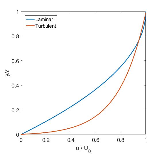
Velocity profile of laminar versus turbulent boundary layer

In the laminar layer, the kinetic energy of the free flowing fluid is transmitted to the slower moving fluid near the surface purely means by of viscosity, i.e. frictional shear stresses. Hence, an imaginary fluid layer close to the free stream pulls along an adjacent layer close to the wall, and so on. As a result, significant portions of fluid in the laminar boundary layer travel at a reduced velocity. In a turbulent boundary layer, the kinetic energy of the free stream is also transmitted via Reynolds stresses, i.e. momentum exchanges due to the intermingling of fluid particles. This leads to a more rapid rise of the velocity away from the wall and a more uniform fluid velocity throughout the entire boundary layer. Due to the presence of the viscous sublayer in the close vicinity of the wall, the wall shear stress in a turbulent boundary layer is governed by the usual equation $\tau = \mu \frac{\mathrm{d}u}{\mathrm{d}y}$ . This means that because of the greater velocity gradient at the wall the frictional shear stress in a turbulent boundary is greater than in a purely laminar boundary layer.

Skin Friction drag

Fluids can only exert two types of forces: normal forces due to pressure and tangential forces due to shear stress. Pressure drag is the phenomenon that occurs when a body is oriented perpendicular to the direction of fluid flow. Skin friction drag is the frictional shear force exerted on a body aligned parallel to the flow, and therefore a direct result of the viscous boundary layer.

Due to the greater shear stress at the wall, the skin friction drag is greater for turbulent boundary layers than for laminar ones. Skin friction drag is predominant in streamlined aerodynamic profiles, e.g. fish, airplane wings, or any other shape where most of the surface area is aligned with the flow direction. For these profiles, maintaining a laminar boundary layer is preferable. For example, the crescent lunar shaped tail of many sea mammals or fish has evolved to maintain a relatively constant laminar boundary layer when oscillating the tail from side to side.

One of Prandtl’s PhD students, Paul Blasius, developed an analytical expression for the shape of a laminar boundary layer over a flat plate without a pressure gradient. Blasius’ expression has been verified by experiments many times over and is considered a standard in fluid dynamics. The two important quantities that are of interest to the designer are the boundary layer thickness $\delta$ and the shear stress at the wall $\tau_w$ at a distance $x$ from the leading edge. The boundary layer thickness is given by

$\delta=\frac{5.2 x}{\sqrt{Re_x}}$

with $Re_x$ the Reynolds number at a distance $x$ from the leading edge. Due to the presence of $x$ in the numerator and $\sqrt{x}$ in the denominator, the boundary layer thickness scales proportional to $x^{1/2}$ , and hence increases rapidly in the beginning before settling down.

Next, we can use a similar expression to determine the shear stress at the wall. To do this we first define another non dimensional number known as the drag coefficient

$C_f=\frac{\tau_w}{1/2 \rho U_f^2}$

which is the value of the shear stress at the wall normalised by the dynamic pressure of the free-flow. According to Blasius, the skin-friction drag coefficient is simply governed by the Reynolds number

$C_f=\frac{0.664}{\sqrt{Re_x}}$

This simple example reiterates the power of dimensionless numbers we mentioned before when discussing wind tunnel testing. Even though the shear stress at the wall is a dimensional quantity, we have been able to express it merely as a function of two non-dimensional quantities $Re$ and $C_f$ . By combining the two equations above, the shear stress can be written as

$\tau_{w}=\frac{0.332 \rho u_f^2}{\sqrt{Re_x}}$

and therefore scales proportional to $x^{-1/2}$ , tending to zero as the distance from the leading edge increases. The value of $\tau_w$ is the frictional shear stress at a specific point $x$ from the leading edge. To find the total amount of drag $D_{sf}$ exerted on the plate we need to sum up (integrate) all contributions of $\tau_w$ over the length of the plate

$D_{sf} = 0.332 \rho U_f^2 \int_0^L \frac{\mathrm{d}x}{\sqrt{Re_x}}=\frac{0.664 \rho U_f^2 L}{\sqrt{\rho U_f L / \mu}} = \frac{0.664 \rho U_f^2 L}{\sqrt{Re_L}}$

where $Re_L$ is now the Reynolds number of the free stream calculated using the total length of the plate $L$ . Similar to the skin friction coefficient $C_f$ we can define a total skin friction drag coefficient $\eta_f$

$\eta_f = \frac{2D_{sf}}{\rho U_f^2 L} = \frac{1.328}{\sqrt{Re_L}}$

Hence, $C_f$ can be used to calculate the local amount of shear stress at a point $x$ from the leading edge, whereas $\eta_f$ is used to find the total amount of skin friction drag acting on the surface.

Unfortunately, do to the chaotic nature of turbulent flow, the boundary layer thickness and skin drag coefficient for a turbulent boundary layer cannot be determined as easily in a theoretical manner. Therefore we have to rely on experimental results to define empirical approximations of these quantities. The scientific consensus of the these relations are as follows:

$\delta = \frac{0.37 x}{(Re_x)^{0.2}}$
$\eta_f = \frac{0.074}{(Re_L)^{0.2}}$

Therefore the thickness of a turbulent boundary layer grows proportional to $x^{4/5}$ (faster than the $x^{1/2}$ relation for laminar flow) and the total skin friction drag coefficient varies as $L^{-1/5}$ (also faster than the $L^{-1/2}$ relation of laminar flow). Hence, the total skin drag coefficient confirms the qualitative observations we made before that the frictional shear stresses in a turbulent boundary layer are greater than those in a laminar one.

Skin friction drag and wing design

The unfortunate fact for aircraft designers is that turbulent flow is much more common in nature than laminar flow. The tendency for flow to be random rather than layered can be interpreted in a similar way to the second law of thermodynamics. The fact that entropy in a closed system only increases is to say that, if left to its own devices, the state in the system will tend from order to disorder. And so it is with fluid flow.

However, the shape of a wing can be designed in such a manner as to encourage the formation of laminar flow. The P-51 Mustang WWII fighter was the first production aircraft designed to operate with laminar flow over its wings. The problem back then, and to this day, is that laminar flow is incredibly unstable. Protruding rivet heads or splattered insects on the wing surface can easily “trip” a laminar boundary layer into turbulence, and preempt any clever design the engineer concocted. As a result, most of the laminar flow wings that have been designed based on idealised conditions and smooth wing surfaces in a wind tunnel have not led to the sweeping improvements originally imagined.

For many years NASA conducted a series of experiments to design a natural laminar flow (NLF) aircraft. Some of their research suggested the wrapping of a glove around the leading edge of a Boeing 757 just outboard of the engine. The modified shape of this wing promotes laminar flow at the high altitudes and almost sonic flight conditions of a typical jet airliner. To prevent the build up of insect splatter at take-off a sheath of paper was wrapped around the glove which was then torn away at altitude. Even though the range of such an aircraft could be increased by almost 15% this, rather elaborate scheme, never made it into production.

In the mid 1990s NASA fitted active test panels to the wings of two F-16’s in order to test the possibility of achieving laminar flow on swept delta-wings flying at supersonic speed; in NASA’s view a likely wing configuration for future supersonic cruise aircraft. The active test panels essentially consisted of titanium covers perforated with millions of microscopic holes, which were attached to the leading edge and the top surface of the wing. The role of these panels was to suck most of the boundary layer off the top surface through perforations using an internal pumping system. By removing air from the boundary layer its thickness decreased and thereby promoted the stability of the laminar boundary layer over the wing. This Supersonic Laminar Flow (SLFC) project successfully maintained laminar flow over a large portion of the wing during supersonic flight of up to Mach 1.6.

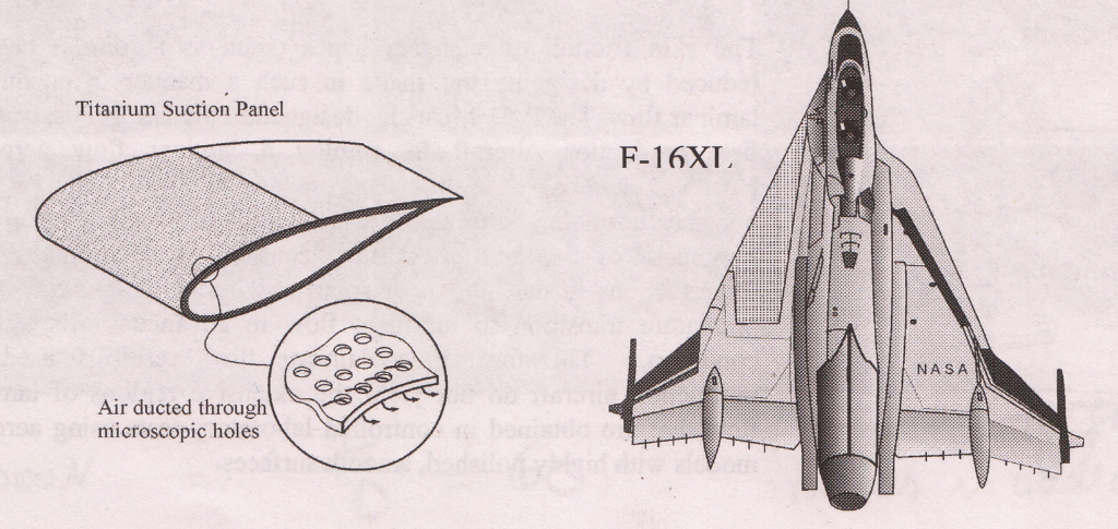
F-16 XL with suction panels to promote laminar flow

While these elaborate schemes have not quite found their way into mass production (probably due to their cost, maintenance problems and risk), laminar flow wings are a very viable future technology in terms of reducing greenhouse gases as stipulated by environmental legislation. An important driver in reducing greenhouse gases is maximising the lift-to-drag ratio of the wings, and therefore I would expect research to continue in this field for some time to come.

19 Responses to On Boundary Layers: Laminar, Turbulent and Skin Friction

Mariette says:

December 12, 2018 at 5:08 pm

Hello,
Thank you very much for this article. I would like to know more about the approximated law given the boundary layer thickness in case of turbulent flow. I mean the law of delta varying with x^4/5.

Can you send me the orogin of your source or the doi of the book/article where you’ve found this relation , please ?

Agian, thank you for your help,

Regards,

Kevin Mariette

Reply
- Rainer says:
  
  December 13, 2018 at 10:14 am
  
  Hi Kevin, thanks for your message. The Wikipedia article has some great sources at the bottom: https://en.wikipedia.org/wiki/Boundary_layer_thickness
  
  The turbulent boundary layer thickness is described in “Boundary-Layer Theory” by Schlichting: https://www.springer.com/gb/book/9783662529171
  
  Hope this helps,
  Rainer
  
  Reply
Aubrey Jaffer says:

January 21, 2019 at 3:10 pm

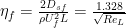
For turbulent flow \eta_f, shouldn’t the exponent of Re_L be 0.2 instead of 0.3?

Reply
- Rainer says:
  
  January 21, 2019 at 3:31 pm
  
  Oh yes, you are absolutely right Aubrey. Thanks for pointing that out. Corrected to 0.2 now.
  
  Reply
David Richardson says:

November 5, 2019 at 5:38 pm

Only a thought but if viscosity is defined by Sutherlands law (I.e a function of temperature) & gamma = cp/cv then doesn’t it follow that the transposed compressible flow equations to define the Mach number will change ? A sensitivitity test would show how much easier it is to “cut through” a hot medium. I guess the question is – is it worth it ? Carrying that extra kit – but leading edges of modern aircraft already have heating elements for deicing – but how long would it take to get the viscosity down. ?

Reply
- Rainer says:
  
  November 6, 2019 at 11:01 am
  
  Hi David,
  
  thanks for your comment. Sure, it would definitely be a matter of a cost-benefit analysis. Intuitively, my first thoughts are that the faster you are going the harder it will be to get heat into the boundary layer to reduce viscosity and skin friction. If the wing is travelling above Mach 1, it’s essentially slicing through the air faster than sound waves travel by bouncing air molecules into each other. By analogy I would presume that conduction, which is also based on molecules boundcing into each other, would be low. That leaves you with convection and radiation but the heat flux into the boundary layer might be so low that it’s just not worth the effort. Here’s a paper from the Journal of Fluid Mechanics that looks into heating the boundary layer.
  
  Cheers,
  Rainer
  
  Reply
  - David Richardson says:
    
    November 6, 2019 at 5:26 pm
    
    Thanks Rainer,
    
    This looks involved- it will take me a while to absorb it all. I was thinking of just making a simple spreadsheet with the derivation of viscosity from Sutherlands law over a range of temperatures (probably air). Plug the resultant viscosities into the derivation of gamma. Plug those gammas into pt/ps=(1+gamma-1/2*m^2)^gamma/gamma -1 transposed to get Mach number & see the resulting change in Mach – just for fun.
    
    Reply
    - David says:
      
      November 6, 2019 at 5:33 pm
      
      Rainer – do you or have you worked in Switzerland- I only ask because I used to work with someone called Rainer over there
      
      Best Regards,
      David
      
      Reply
    - Rainer says:
      
      November 6, 2019 at 7:13 pm
      
      Hi David,
      yes, absolutely. That would be the simplest and quickest way to get a feel for how the viscosity changes the Mach number for a given pressure ratio (and fun of course). But I guess the question remains could you actually get sufficient heat flux into the air with something like a de-icing device to cause an appreciable change in temperature? I guess the fluid right at the surface of the wing will take the temperature of the heating device, but then it might drop off quite dramatically moving away from the surface.
      
      Ha, no I have never worked in Switzerland. But Rainer is a common name in the German-speaking world, so there will be plenty of others with the same name 🙂
      
      Reply
      - David says:
        
        November 6, 2019 at 7:58 pm
        
        Oh right – chap I used to work with was from Baden named Rainer – didn’t know it was a popular name on the continent- forgive my ignorance.
        
        Yes just a quick bit of fun – hypothetical of course- because as you rightly pointed out:
        
        1) what’s the sensitivity (does it make “bugger all difference”
        2) how can you heat it up
        3)how long will it take to heat it up
        4) how long will the heat be retained keeping the viscosity low over the body ?
        
        My brother is a laser engineer in the states- but I can’t see this being a practical solution. Heating elements across the body?
        
        Like I said just a bit of fun.
        
        Best Regards,
        David
        
        P.s. do you have a LinkedIn account?
      - Rainer says:
        
        November 6, 2019 at 8:40 pm
        
        Nothing to apologise for David 🙂
        
        Might make it even more fun by extending the back-of-the-envelope calculation to convection/conduction. Given a certain wing skin temperature, how much can you expect to heat up the surrounding fluid?
        
        My LinkedIn account is the following: https://www.linkedin.com/in/rainergroh/
David says:

November 6, 2019 at 9:44 pm

Not really sure to be honest ht=mcpdeltat so I guess the speed is critical for heat pickup – like I said just fun really – suppose I could pick up one of my old cfd models and change the body temperature by a number of increments to get an empirical relationship.

P.s I’ve tried to link in with you

Best Regards,
David

Reply
Robert says:

May 12, 2020 at 3:51 am

Nice article, had some good formulas in there that are important for calculating drag.

I just have a quick question do you calculate a drag coefficent based on combined boundary layer flow, so laminar going to turbulent flow ?
I am confused on how you can calculate a drag coefficient based for this.

Reply
Robert says:

May 12, 2020 at 4:03 am

Just a correction to my previous comment, my question is meant to read

How do you calculate a drag coefficent based on combined boundary layer flow, so laminar going to turbulent flow ?

Reply
- Rainer says:
  
  May 14, 2020 at 7:51 am
  
  Hi Robert, thanks for your comment. An expression for the skin friction drag coefficient in transitional flow can actually be found on Wikipedia: https://en.wikipedia.org/wiki/Skin_friction_drag#Transitional_flow
  
  Reply
Thomas R Norris says:

April 4, 2022 at 8:48 pm

Very nice article, fun to read. Question: Is the laminar-to-turbulent transition number range give just for pipe flow, where the characteristic Re the diameter? The plate example from what I read transitions around Re = 600,000.
I greatly enjoyed the way you explained the many aerodynamic items without getting too mathematical. That is hard to do. Thank you!

Reply
- Rainer says:
  
  April 5, 2022 at 8:00 am
  
  Dear Thomas, the laminar to turbulent transition for a flat plate is around 5×10^5, I believe. For pipe flow it is much lower, in the range of 2×10^3.
  
  Reply
Wall Function: Boundary Layer Modelling Approach - All About CFD... says:

June 3, 2022 at 6:59 am

[…] On September 20, 2021June 3, 2022 By rajatwalia1997In Tom's Posts – "All About CFD…" Reference: aerospaceengineeringblog […]

Reply
Antar abdala says:

December 22, 2022 at 8:50 pm

Rayleigh number if we are speaking about free convection in smoke rising from a cigarette, instead of Reynolds number

Reply